# Load necessary libraries
library(tidyverse)
library(here)
library(janitor)
library(sf)
library(ggspatial)
library(prettymapr)
library(showtext)
library(ggalluvial)
# Add desired fonts
font_add_google(name = "Noto Sans", family = "noto_sans")
font_add_google("Libre Baskerville", family = "libre")
# Load in data and standardize column names
light_pol <- read.delim(here("posts", "ermine_moth_infographic", "data", "light_pol.txt"), skip = 2) %>%
clean_names() %>%
# Separate location column
separate_wider_delim(
cols = location_country,
delim = "/",
names = c("loc_name", "country")
) %>%
# Remove any white space from separated columns
mutate(country = str_squish(country), loc_name = str_squish(loc_name)) %>%
# Rename population column to be more relevant
rename(pollution_status = population) %>%
# Recode values to be more intuitive
mutate(
pollution_status = recode(
pollution_status,
"dark-sky" = "non polluted",
"light-polluted" = "polluted"
),
# Recode country codes to full names
country = recode(country, "F" = "France", "CH" = "Switzerland"),
# Fix location name with conversion error
loc_name = recode(loc_name, "Kleinl�tzel" = "Kleinlützel")
) %>%
# Make a new column with pollution bin values
mutate(
pollution_bin = case_when(
loc_name == "Blochmont" ~ "0.25–0.4",
loc_name == "Kleinlützel" ~ "0.4-1",
loc_name == "Kiffis" ~ "0.4-1",
loc_name == "Doucier" ~ "0.4-1",
loc_name == "Lutterbach" ~ "1-3",
loc_name == "Allschwil" ~ "20-40",
loc_name == "Reinach" ~ "20-40",
loc_name == "Hegenheim" ~ ">40",
loc_name == "Basel Kannenfeld" ~ ">40",
loc_name == "Basel Spalentor" ~ ">40"
),
# New Latitude and Longitude column with values from paper
lat = case_when(
loc_name == "Blochmont" ~ 47 + 26 / 60 + 16 / 3600,
loc_name == "Kleinlützel" ~ 47 + 25 / 60 + 55 / 3600,
loc_name == "Kiffis" ~ 47 + 26 / 60 + 18 / 3600,
loc_name == "Doucier" ~ 46 + 39 / 60 + 40 / 3600,
loc_name == "Lutterbach" ~ 47 + 46 / 60 + 12 / 3600,
loc_name == "Allschwil" ~ 47 + 32 / 60 + 52 / 3600,
loc_name == "Reinach" ~ 47 + 31 / 60 + 50 / 3600,
loc_name == "Hegenheim" ~ 47 + 33 / 60 + 43 / 3600,
loc_name == "Basel Kannenfeld" ~ 47 + 33 / 60 + 59 / 3600,
loc_name == "Basel Spalentor" ~ 47 + 33 / 60 + 28 / 3600
),
lon = case_when(
loc_name == "Blochmont" ~ 7 + 14 / 60 + 10 / 3600,
loc_name == "Kleinlützel" ~ 7 + 22 / 60 + 57 / 3600,
loc_name == "Kiffis" ~ 7 + 17 / 60 + 59 / 3600,
loc_name == "Doucier" ~ 5 + 41 / 60 + 21 / 3600,
loc_name == "Lutterbach" ~ 7 + 3 / 60 + 36 / 3600,
loc_name == "Allschwil" ~ 7 + 32 / 60 + 8 / 3600,
loc_name == "Reinach" ~ 7 + 36 / 60 + 25 / 3600,
loc_name == "Hegenheim" ~ 7 + 31 / 60 + 14 / 3600,
loc_name == "Basel Kannenfeld" ~ 7 + 34 / 60 + 19 / 3600,
loc_name == "Basel Spalentor" ~ 7 + 34 / 60 + 53 / 3600)) %>%
mutate(pollution_bin = factor(pollution_bin, levels = c("0.25–0.4",
"0.4-1",
"1-3",
"20-40",
">40")
)
)
# Create sf object for mapping
light_pol_sf <- st_as_sf(light_pol, coords = c("lon", "lat"), crs = 4326)
# Enable font interp
showtext_auto(enable = TRUE)
# Create map
ggplot(light_pol_sf) +
# Use OpenStreetMap basemap
annotation_map_tile(type = "cartodark", zoomin = 0) +
# Fill points by radiance measured
geom_sf(
aes(fill = pollution_bin),
color = "white",
size = 6,
shape = 21
) +
# Create custom radiance color scale
scale_fill_manual(values = c("#893533", "#AE4716", "#F6A905", "#FFF533", "#FFFCC2")) +
# Add labels
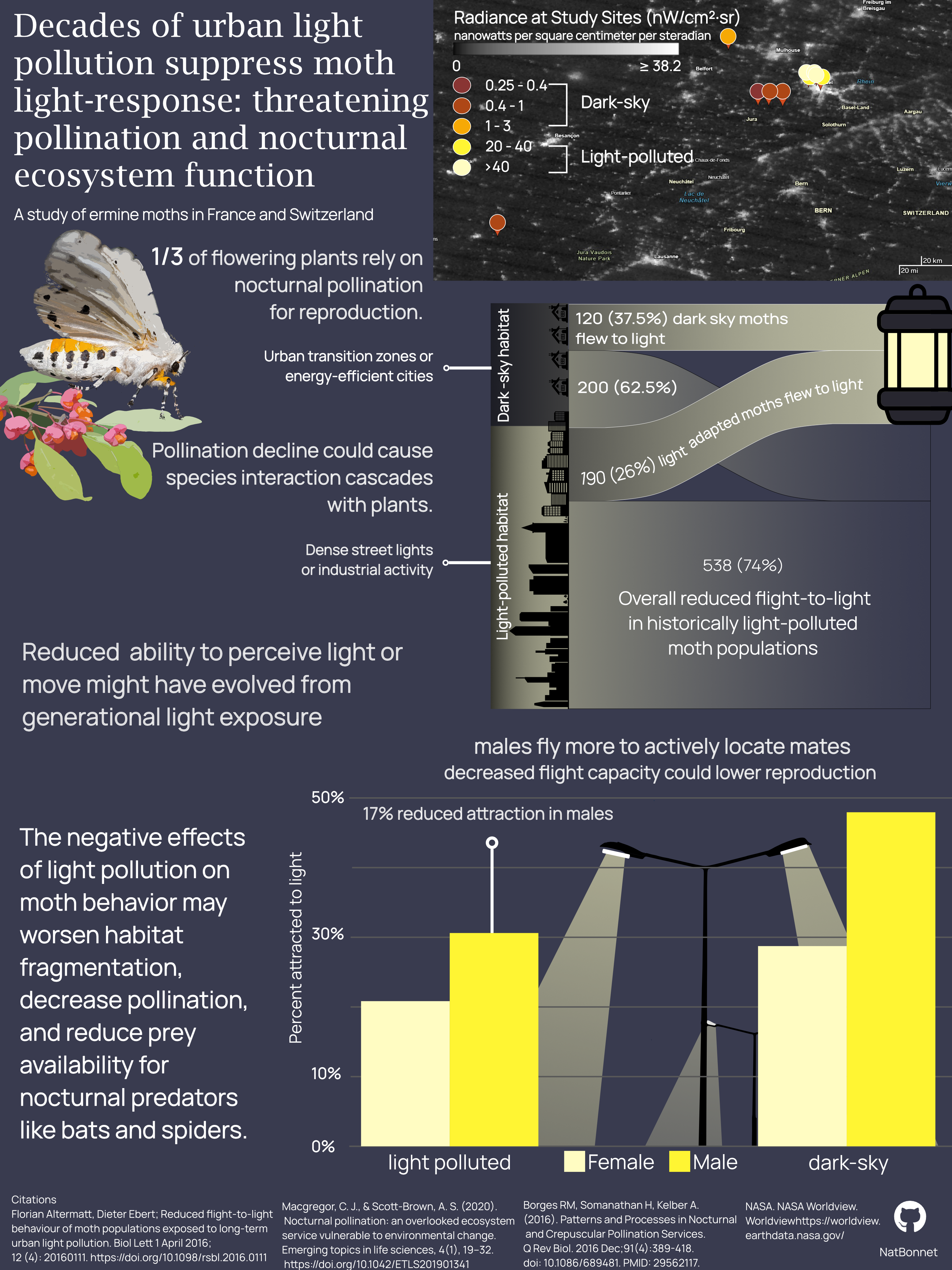
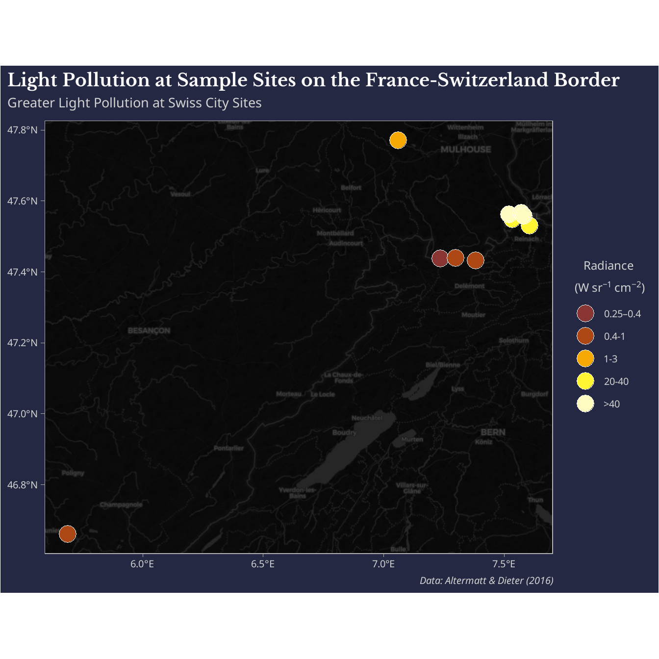
labs(title = "Light Pollution at Sample Sites on the France-Switzerland Border",
subtitle = "Greater Light Pollution at Swiss City Sites",
caption = "Data: Altermatt, Florian; Ebert, Dieter (2016)") +
theme_light() +
# Add legend title
guides(fill = guide_legend(
# Legend title
title = "Radiance\n(10–9 W sr–1 cm–2)"
)) +
# Create custom theme
theme(
plot.background = element_rect(fill = "#242842"),
panel.background = element_rect(fill = "#242842"),
legend.background = element_rect(fill = "#242842"),
# Align with y axis text instead of just axis
plot.title.position = "plot",
# Edit title format
plot.title = element_text(
face = "bold",
family = "libre",
size = 27,
lineheight = 1.5,
color = "white"),
# Subtitle format
plot.subtitle = element_text(
family = "noto_sans",
size = 20,
margin = margin(b = 8),
color = "lightgrey"),
# Axis labels
axis.text = element_text(size = 15,
family = "noto_sans",
color = "lightgrey"),
# Caption format
plot.caption = element_text(
family = "noto_sans",
face = "italic",
size = 15, color = "lightgrey"),
# Legend text and title format
legend.text = element_text(size = 15,
family = "noto_sans", color = "lightgrey"),
legend.title = element_text(size = 18,
family = "noto_sans", color = "lightgrey")
)
# Create pollution summary by status and sex- with proportion for attraction
pol_sum <- light_pol %>%
group_by(pollution_status, sex) %>%
summarise(
total_attracted = sum(moths_attracted),
total_not_attracted = sum(moths_not_attracted),
prop_attracted = total_attracted / (total_attracted + total_not_attracted)
) %>%
# Add better labels for sex
mutate(pollution_status = factor(pollution_status, levels = c("polluted", "non polluted")),
sex = recode(sex,
"m" = "Male",
"f" = "Female"))
# Bar plot
ggplot(pol_sum, aes(x = pollution_status, y = prop_attracted, fill = sex)) +
# Put sex columns next to each other instead of stacking
geom_col(position = "dodge") +
# Fill labels to look like light beams
scale_fill_manual(values = c("#FFFCC2", "#FFF533")) +
scale_y_continuous(labels = scales::percent)+
# Add labels
labs(title = "Flight-to-Light Behavior in Ermine Moths",
subtitle = "Moths in light polluted areas show reduced attraction to light",
caption = "Data: Altermatt, Florian; Ebert, Dieter (2016)",
y = "Proportion of moths attracted to light")+
theme_minimal() +
# Apply custom theme
theme(
# Move legend to the bottom of the plot
legend.position = "bottom",
# Remove axis title because it's redundant
axis.title.x = element_blank(),
# Background colors
plot.background = element_rect(fill = "#242842"),
panel.background = element_rect(fill = "#242842"),
legend.background = element_rect(fill = "#242842"),
# Align with y axis text instead of just axis
plot.title.position = "plot",
# Title
plot.title = element_text(
face = "bold",
family = "libre",
# Size relative to base size in theme
size = 27,
lineheight = 1.5,
color = "white"
),
# Subtitle
plot.subtitle = element_text(
family = "noto_sans",
size = 20,
margin = margin(b = 8),
color = "lightgrey"
),
# Axis titles
axis.title = element_text(
size = 15,
family = "noto_sans",
color = "lightgrey"
),
# Axis labels
axis.text = element_text(
size = 15,
family = "noto_sans",
color = "lightgrey"
),
# Caption
plot.caption = element_text(
family = "noto_sans",
face = "italic",
size = 15,
color = "lightgrey"
),
# Legend
legend.text = element_text(
size = 15,
family = "noto_sans",
color = "lightgrey"
),
legend.title = element_blank()
)
# Create dataframe for overall summary proportions
pol_tot_sum <- light_pol %>%
group_by(pollution_status) %>%
summarise(
total_attracted = sum(moths_attracted),
total_not_attracted = sum(moths_not_attracted),
prop_attracted = total_attracted / (total_attracted + total_not_attracted)
)
# Create a pivoted data frame to summarize attraction trends
df <- pol_tot_sum %>%
# Remove the proportion column
select(-prop_attracted) %>%
pivot_longer(
# Pivot attracted and unattracted to one column called 'attraction'
cols = c(total_attracted, total_not_attracted),
names_to = 'attraction' ,
# Summarize all count values
values_to = 'count'
) %>%
# Recode for nicer plot output
mutate(attraction = recode_factor(attraction,
total_attracted = "attracted",
total_not_attracted = "not attracted"))
# Create alluvial diagram using ggalluvial package
alluvial_plot <- ggplot(df,
aes(axis1 = pollution_status, axis2 = attraction, y = count)) +
geom_alluvium(aes(fill = pollution_status), width = 0.3, alpha = 0.7) +
geom_stratum(width = 0.2, fill = "white", color = "grey60") +
geom_text(stat = "stratum", aes(label = after_stat(stratum)),
size = 3.5) +
scale_fill_manual(values = c("#868677", "#535459")) +
scale_x_discrete(limits = c("Pollution Status", "Attraction"),
expand = c(0.1, 0.1)) +
labs(y = "Number of moths") +
theme_minimal() +
theme(legend.position = "none") +
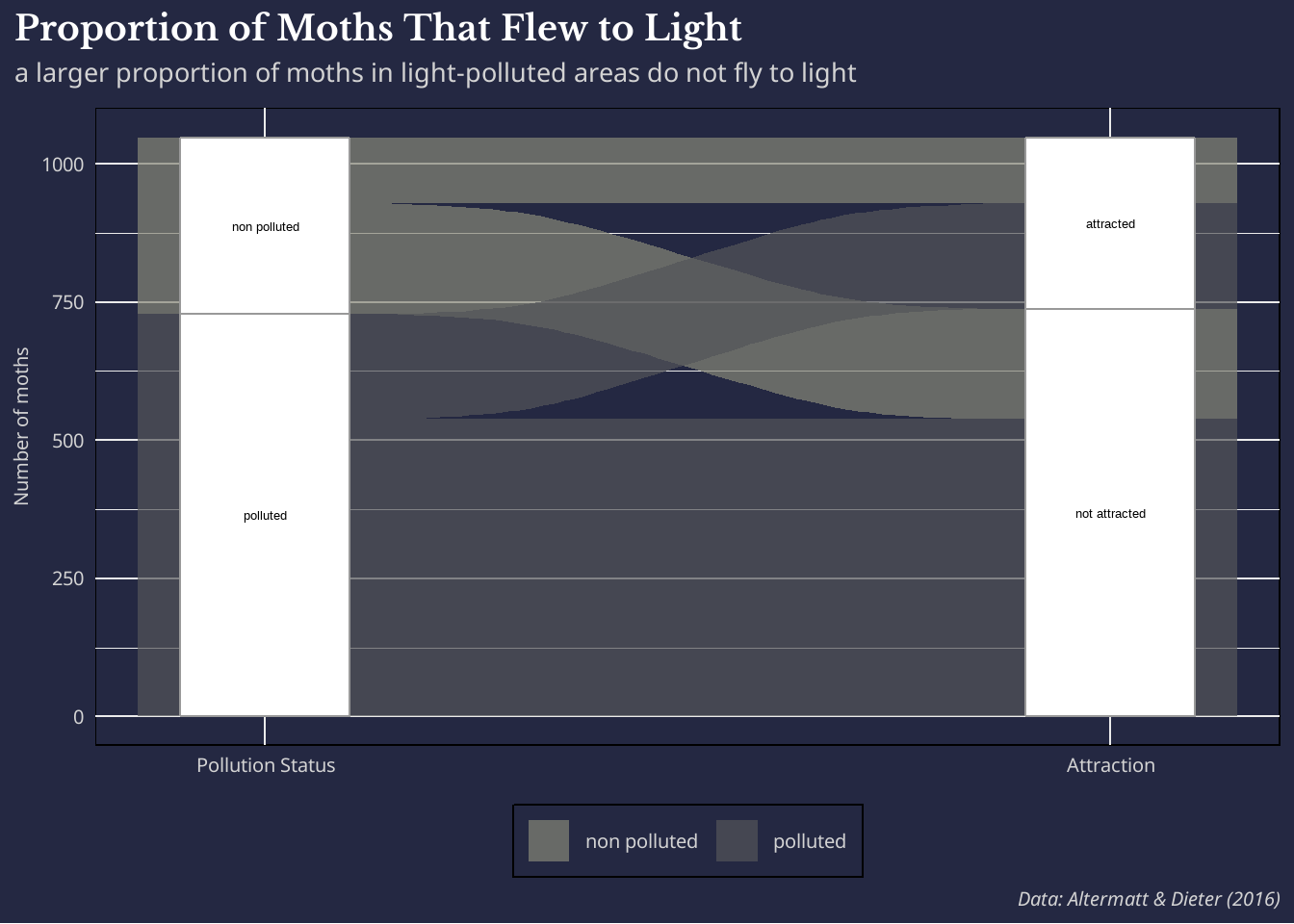
labs(title = "Proportion of Moths That Flew to Light",
caption = "Data: Altermatt, Florian; Ebert, Dieter (2016)",
subtitle = "a larger proportion of moths in light-polluted areas do not fly to light") +
theme(
# Move legend to the bottom of the plot
legend.position = "bottom",
# Remove axis title because it's redundant
axis.title.x = element_blank(),
# Background colors
plot.background = element_rect(fill = "#242842"),
panel.background = element_rect(fill = "#242842"),
legend.background = element_rect(fill = "#242842"),
# Align with y axis text instead of just axis
plot.title.position = "plot",
# Title
plot.title = element_text(
face = "bold",
family = "libre",
# Size relative to base size in theme
size = 27,
lineheight = 1.5,
color = "white"
),
# Subtitle
plot.subtitle = element_text(
family = "noto_sans",
size = 20,
margin = margin(b = 8),
color = "lightgrey"
),
# Axis titles
axis.title = element_text(
size = 15,
family = "noto_sans",
color = "lightgrey"
),
# Axis labels
axis.text = element_text(
size = 15,
family = "noto_sans",
color = "lightgrey"
),
# Caption
plot.caption = element_text(
family = "noto_sans",
face = "italic",
size = 15,
color = "lightgrey"
),
# Legend
legend.text = element_text(
size = 15,
family = "noto_sans",
color = "lightgrey"
),
legend.title = element_blank()
)


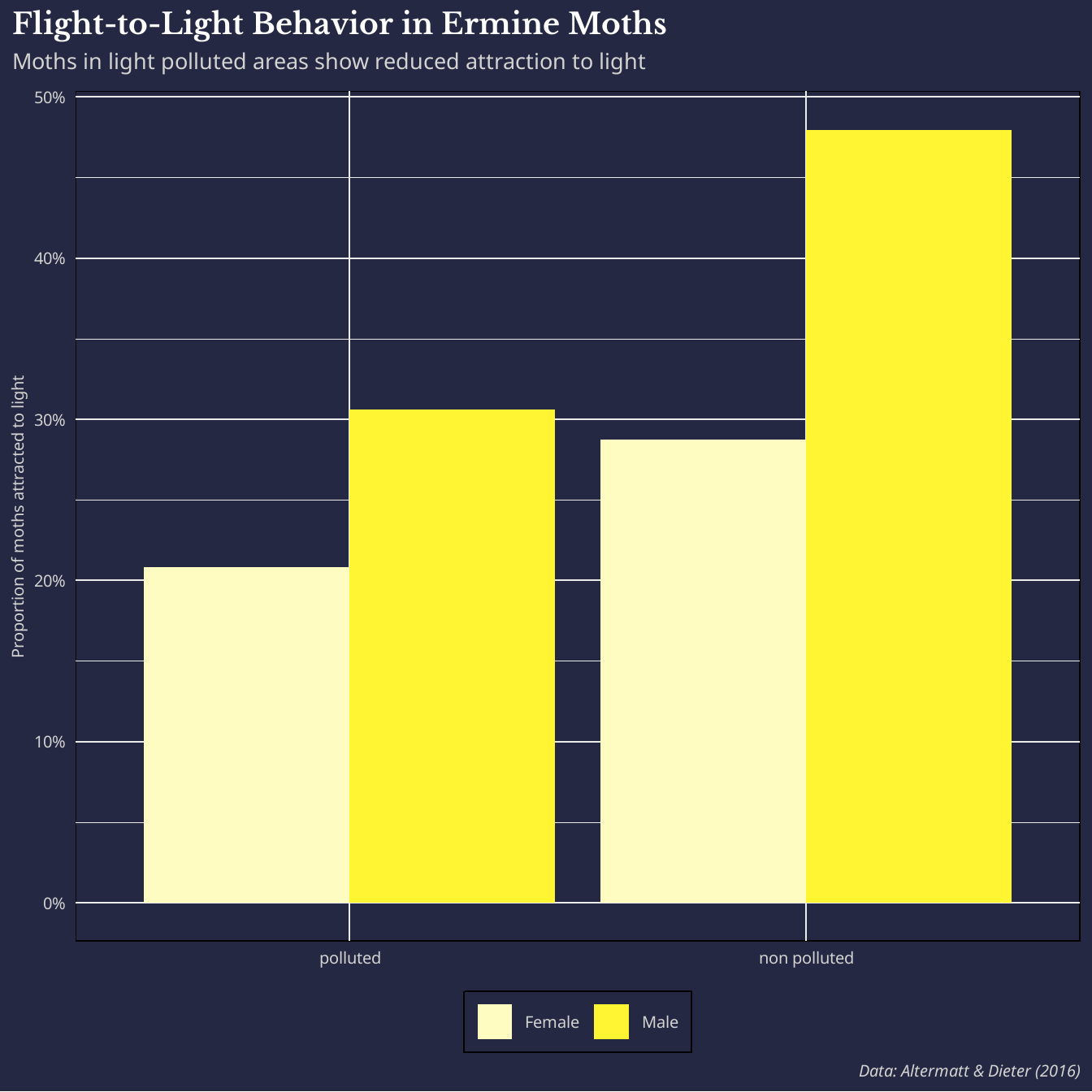 This bar chart is essentially a recreation of the study’s main figure with tweaks for interpretability.